Stage 03 · Scaling data
Sharding & Partitioning
One machine stopped being enough. You need to split your data across several. The whole question is: split it on what?
The instinctive answer — “something that spreads the load evenly” — is usually wrong, and this note is about why.
Start with the obvious one
Say you’re storing events for a ticketing site, and one database is no longer coping. The simplest split is to hash the key and take a modulo:
database_id = hash(event_id) % number_of_databasesEvent 1234 hashes to database 1, event 5678 to database 0, and so on. Load spreads beautifully — hash functions are good at that. Every lookup by event_id goes to exactly one machine.
This is a fine design, right up until you ask it a question with a range in it.
“Give me all events in March.” There’s no March shard. Events from March are scattered uniformly across every machine you own, because that’s precisely what hashing was for. So you ask all of them and merge.
“Give me all events near this venue.” Same thing. Physical proximity means nothing to a hash function.
You optimised for write distribution and paid for it with every read that isn’t a point lookup.
The test that catches this
Here’s a question worth asking of any sharding scheme:
As I add nodes, does this query touch more of them?
For a point lookup by the shard key: no. One shard, forever, whether you have three machines or three thousand.
For our March query: yes. Ten shards means ten round-trips. A thousand shards means a thousand. You added machines to handle more load and made your reads worse.
That’s the difference between bounded and unbounded fan-out, and it matters more than almost anything else in a sharding decision.
Bounded fan-out is fine. “This query touches three shards because the search radius spans three cells” is healthy — it stays three whether you run a hundred machines or a hundred thousand.
Unbounded fan-out is a trap. Your p99 latency becomes the p99 of the slowest of N responses, so a one-in-a-thousand slow shard starts appearing in essentially every query once you have a thousand shards. This is tail latency amplification and it gets worse exactly as you grow.
So: choose the key from the query, not the load
The selection procedure, in three steps:
- Name your highest-QPS query and your highest-correctness query. They’re often different.
- Pick the key that makes those single-shard.
- Then look at load balance — and if it’s uneven, fix it by splitting shards, not by changing the key.
That ordering is the whole discipline. Load imbalance has several fixes (Hotspots and Dynamic Resharding). A shard key that destroys locality has none.
The four strategies
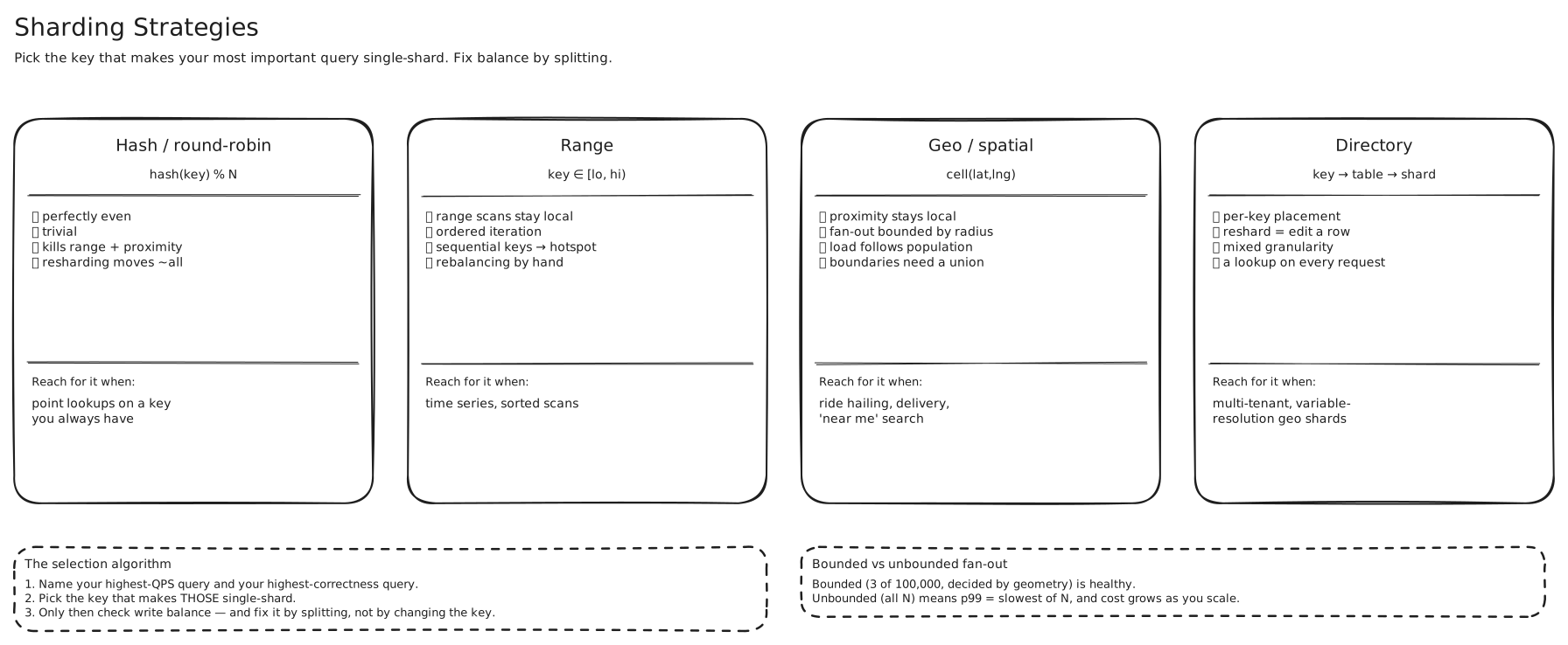
Hash / round-robin. hash(key) % N. Perfectly even, trivially simple, and destroys every range and proximity query. Resharding moves nearly everything unless you use consistent hashing. Right for point lookups on a key you always have: sessions, user profiles, key-value caches.
Range. key ∈ [lo, hi) → shard. Range scans hit few shards; ordered iteration works. But sequential keys — timestamps, auto-increment ids — send every new write to the last shard, and rebalancing means hand-picking new boundaries. Right for time series and sorted scans.
Geo / spatial. cell(lat, lng) → shard. Proximity reads stay local and fan-out is bounded by the search radius rather than the cluster size. The cost: load follows population, so hotspots are guaranteed, and queries near a cell boundary need a union of shards. Right for anything with a “near me” query.
Directory / lookup. key → table → shard. The mapping is stored rather than computed. Arbitrary per-key placement, mixed granularity, and resharding becomes editing a row. The cost is a lookup on every request, plus a new consistency question about that lookup. Right for multi-tenant systems, and for anything where you need to do surgery on hot keys.
Horizontal, vertical, and the three things people call “vertical”
Everything above splits rows. Event 1234 lives on one machine, event 5678 on another, and both machines have the identical schema. That’s horizontal partitioning, and when someone says “sharding” with no qualifier, this is what they mean.
Vertical partitioning splits columns. Look at the events table again:
events(event_id, title, venue_id, starts_at, seatmap JSONB)Every request reads title and starts_at. Almost nothing reads seatmap, which is 200 KB of nested JSON. But the database stores the whole row together, so that blob is sitting on the same page as the columns you actually want, and your buffer pool is full of seatmaps nobody asked for.
Split it:
events(event_id, title, venue_id, starts_at)
event_seatmaps(event_id, seatmap)
Now the hot row is tiny, far more rows fit per page, and a much larger fraction of your working set stays in memory. You didn’t add a machine — you made the machine you have go further.
That difference matters, so be precise about it: vertical partitioning raises a ceiling, horizontal partitioning removes one. Narrowing rows makes each read cheaper. It does not give you a second machine’s worth of write throughput, and no amount of it will.
Two more things wear the word “vertical”, and mixing them up is the actual source of the confusion:
- Vertical scaling is buying a bigger machine. Nothing to do with columns.
- Federation (functional partitioning) splits whole tables across databases by feature — users here, events there, payments somewhere else. People often call this vertical partitioning, and you’ll survive, but it’s a different operation on a different axis. → Database Federation
One last piece of vocabulary worth nailing down, because it trips people in interviews: partitioning is not sharding. Postgres PARTITION BY RANGE (starts_at) splits one logical table into many physical ones — on the same server. You get smaller indexes and cheap partition drops for retention, and zero extra machines. Sharding is what you call it when the partitions live on different servers and the application has to figure out which one to talk to.
Algorithmic versus directory sharding
The first three are algorithmic: the shard is a pure function of the key. No lookup, no state, nothing to keep consistent — and no flexibility. Every key in the space is treated identically.
The moment you want different keys placed by different rules — this region finely divided, that one coarsely; this tenant isolated on its own machine — the rule stops being computable and has to be stored. That’s directory sharding, and it’s a real architectural shift, not a detail.
It’s worth naming what you gain: putting the placement rule in data instead of in code means resharding is an UPDATE, not a deploy. That single property is what makes adaptive schemes possible at all.
Then cache the directory aggressively, because you’re now reading it constantly — and decide, per code path, whether a stale routing decision is survivable. → Caching Strategies, Replication and Read Consistency
Three things the shard key decides for you
You get exactly one cheap access path. Every other way of querying the table is either a scatter-gather or a separate structure you maintain yourself. → Secondary Indexes at Scale
It decides how hard your concurrency control is. If everyone competing for the same decision lands on the same shard, a single-row conditional update is atomic by definition — no lock service, no consensus. If they land on different shards, you need real distributed coordination. Choosing the shard key is choosing how difficult this will be. → Avoiding Distributed Transactions
It creates your cross-shard write problem. Two rows on two shards can’t be written atomically without two-phase commit. The usual escape is to order them so the only reachable inconsistency is harmless. → Avoiding Distributed Transactions
What sharding costs you
Everything so far has been about picking the key well. This section is about the bill that arrives even when you pick it perfectly — because a sharded database is a meaningfully weaker database than the one you started with, and knowing exactly which powers you gave up is most of the skill.
Joins stop being free
On one machine, events JOIN venues ON events.venue_id = venues.venue_id is a query the planner optimises for you. Shard events by event_id and venues by venue_id and those two rows are on different machines. The planner can’t help; there is no plan.
You have three ways out, and you’ll use all three eventually.
Denormalise. Copy venue_name into the events row. The join disappears because the data is already there. You now own the problem of keeping the copy correct when a venue is renamed. → Normalization and Denormalization
Replicate the small side everywhere. A venues table of fifty thousand rows fits comfortably on every shard. Ship a full copy to each one and the join becomes local again. This works beautifully for small, slow-changing reference data and not at all for anything large or hot.
Join in the application. Fetch the events, collect the distinct venue_ids, one batched read to the venue shards, stitch. Two round trips instead of one, and it’s on you to keep the fan-out bounded.
Transactions stop being free
Two rows on two machines can’t be updated atomically without two-phase commit, which means a coordinator, locks held across a network hop, and an availability story that’s worse than either database alone. Most systems refuse to pay that and restructure the problem instead — order the writes so the only reachable intermediate state is harmless, or make the operation idempotent and retry. → Avoiding Distributed Transactions, Idempotency
Aggregation becomes scatter-gather
SELECT COUNT(*) FROM events WHERE status = 'on_sale' used to be one query. Now it’s N queries and a sum, with your latency set by the slowest shard.
Some aggregates decompose cleanly: COUNT, SUM, MIN, MAX, and AVG if you carry the count along with the sum. Some don’t. COUNT(DISTINCT user_id) is the one that bites — you can’t add up per-shard distinct counts, because the same user may appear on several shards. Either you ship all the ids to one place, or you accept an approximation from a sketch like HyperLogLog.
Ordering is the other trap. Global top-10 is fine: ask each shard for its top 10 and merge, which is a genuinely correct algorithm. ORDER BY ... LIMIT 10 OFFSET 10000 is not fine, because to skip 10,000 rows globally you need 10,010 rows from every shard. Deep pagination and exact global percentiles are where fan-out queries go to die.
The usual real answer is to stop asking the sharded store these questions at all. Stream changes out to a warehouse or a search index and aggregate there, or maintain counters incrementally as writes happen.
Global uniqueness is gone
This one surprises people. AUTO_INCREMENT and SERIAL are per-database. Shard 0 and shard 1 will both cheerfully hand out id 1, and now you have two different events with the same primary key.
UNIQUE(email) has the same problem. The constraint is enforced per shard, so unless email is your shard key, two shards will each happily accept the same address. Global uniqueness becomes an application concern, usually a separate small table that acts as a claim registry.
For ids specifically, there are three standard answers.
UUIDs. 128 bits, generated anywhere, no coordination at all. The cost is size — Instagram ruled them out partly on storage, at 96 bits and up versus the 64 they wanted — and, more painfully, that random UUIDv4s have no time ordering, so every insert lands on a random B-tree page and your index write locality is destroyed. UUIDv7 (standardised in RFC 9562) puts a millisecond timestamp in the high bits specifically to fix that.
Snowflake ids. Pack a 64-bit integer out of a timestamp, a generator id, and a per-millisecond sequence. You get something that fits in a BIGINT, sorts roughly by creation time, and needs no coordination beyond making sure each generator has a distinct id. Instagram’s variant is worth memorising because it’s so concrete: 41 bits of millisecond timestamp, 13 bits of logical shard id, 10 bits of sequence (so 1,024 ids per shard per millisecond), against a custom epoch of 1 January 2011 — and they implemented it as a stored procedure inside Postgres rather than running a separate ID service. The catch is that you now depend on clocks: a generator whose clock jumps backwards can reissue ids.
Ticket servers. One tiny dedicated database whose only job is an auto-increment counter. Flickr famously ran two of them, one issuing odd numbers and one issuing even, so neither was a single point of failure. Dead simple and gives you small sequential integers, but it’s a network hop on every insert and another thing to keep alive. Hand out blocks of a thousand ids at a time and the hop mostly goes away.
| Coordination needed | Time-sortable | Size | Main cost | |
|---|---|---|---|---|
| UUIDv4 | none | no | 128 bits | random index writes, storage |
| Snowflake | assign each generator an id | yes | 64 bits | depends on clocks |
| Ticket server | a live central service | yes | 64 bits | extra hop, extra thing to run |
Notice the sneaky benefit in the middle row: if you put the shard id inside the id, then the id tells you where the row lives. No directory lookup, no second query. That’s why Instagram spent 13 of their 64 bits on it.
And then there’s rebalancing
Shards don’t stay even. Data grows unevenly, traffic grows very unevenly, and eventually you’re moving keyspace around while the system is serving traffic. How much that hurts depends entirely on the scheme you picked — which is the next section — and how often you have to do it depends on how skewed your keys are. → Consistent Hashing, Hotspots and Dynamic Resharding
Resharding
Eventually the shape you chose stops fitting. What that costs depends entirely on the scheme:
| Scheme | What a reshard costs |
|---|---|
| Naive modulo hash | changing N remaps nearly every key |
| Consistent hashing | only about K/N keys move; virtual nodes even out the result |
| Range split | pick a new boundary — but neighbours often need adjusting too, since ranges must tile exactly |
| Hierarchical key split | subdivide one key into its children; hashing places them for you |
That last row is worth planning for. If you expect to reshard often, prefer a key space with a built-in subdivision rule — a quadtree cell, an H3 cell, a tenant that can split into sub-tenants. “Split this cell into its seven children and let hashing redistribute them” is a much simpler operation than “recompute boundaries for this shard and the two next to it.” → Hotspots and Dynamic Resharding
In an interview
Derive the shard key from the query, out loud. “We read this three ways and can only shard on one — let’s try this key and see what happens to the other queries” is much stronger than announcing a key.
Use the fan-out test when defending it: as I add nodes, does this query touch more of them? It’s a crisp way to show why a key is right or wrong.
The trap is sharding too early. Say you’d exhaust replicas, caching, indexes and federation first, because sharding is the one step that’s hard to reverse.
Seen in
- 08 - Location Index Scaling Problem — round-robin sharding a geo index, and both ways it fails
- 09 - H3 and Geo Sharding — a hierarchical spatial cell as the shard key
- 03 - Data Model and Sharding — one table read three ways, and only one key to shard on
Related
Geospatial Indexing · Hotspots and Dynamic Resharding · Secondary Indexes at Scale · Avoiding Distributed Transactions