Stage 01 · Foundations
Availability
Availability is the fraction of time your system actually answers. It looks like a number you get to choose, and it isn’t — it’s an arithmetic consequence of how many things you depend on, how often each one breaks, and how fast you get it back.
“We’re up 99.9% of the time.” Is that good?
You’re running an online store. Catalogue, cart, checkout, the usual. Someone asks what your uptime is and you say 99.9%. Three nines. It sounds excellent.
Then do the arithmetic. A year is 8,760 hours. One tenth of one percent of that is 8.76 hours — a full working day, every year, where nobody can buy anything. If it all lands on Black Friday, that’s not a metric, that’s a resignation letter.
This is the one place a table earns its keep, because the whole lesson is in reading down the column.
| Availability | Downtime per year | Per 30 days | Per week |
|---|---|---|---|
| 90% (“one nine”) | 36.5 days | 3 days | 16.8 hours |
| 99% | 3.65 days | 7.2 hours | 1.68 hours |
| 99.9% | 8.76 hours | 43.2 minutes | 10.1 minutes |
| 99.95% | 4.38 hours | 21.6 minutes | 5.04 minutes |
| 99.99% | 52.6 minutes | 4.32 minutes | 60.5 seconds |
| 99.999% | 5.26 minutes | 25.9 seconds | 6.05 seconds |
Each extra nine divides your downtime budget by ten. It does not divide the cost by anything — it multiplies it. Google’s SRE book is blunt about this: past a certain point “an incremental improvement in reliability may cost 100x more than the previous increment,” and users often can’t tell the difference anyway because their own phone and their own wifi are less reliable than your service.
Look at the “per week” column and you’ll see something practical. At 99.99%, your entire weekly budget is one minute. A human being cannot get paged, wake up, open a laptop and fix something in one minute. Four nines and up is a statement about your automation, not about your on-call rota.
Where the downtime actually comes from
Two numbers produce that percentage. MTBF, mean time between failures, is how often the thing breaks. MTTR, mean time to recovery, is how long it stays broken. Availability is the ratio of working time to total time:
A = MTBF / (MTBF + MTTR)Say your checkout service falls over roughly once a month, and a human takes four hours to notice, diagnose and fix it.
MTBF = 720 h   (30 days)
MTTR = 4 h
A    = 720 / 724 = 0.9945   →  99.45%,  about 48 hours down per year
Two nines and a bit. You now have exactly two dials.
Turn the MTBF dial: make it break half as often. More tests, more review, fewer risky deploys. That’s slow, expensive work, and it buys you 1440/1444 = 99.72% — about 24 hours a year. You halved your failure rate and you still aren’t at three nines.
Turn the MTTR dial instead. Same buggy code, same failure rate, but a health check notices in ten seconds and the orchestrator replaces the instance before a human is even paged.
MTBF = 720 h
MTTR = 5 min = 0.083 h
A    = 720 / 720.083 = 0.99988   →  99.99%,  about 1 hour down per year
Identical number of failures. Four nines instead of two. MTTR is nearly always the cheaper dial, because automation can move it by a factor of fifty and nothing you do will make your code fifty times less buggy. This is why so much availability work is really detection and recovery work: health checks, fast rollback, automated failover, circuit breakers that fail a call in 50ms instead of hanging for 30 seconds. → Circuit Breakers
Every dependency you add spends availability
Now let’s stop talking about one service. Your store’s checkout path looks like this:
client → load balancer → app server → databaseAll three have to work for a checkout to succeed. Suppose each is independently up 99.9% of the time. What’s the availability of checkout?
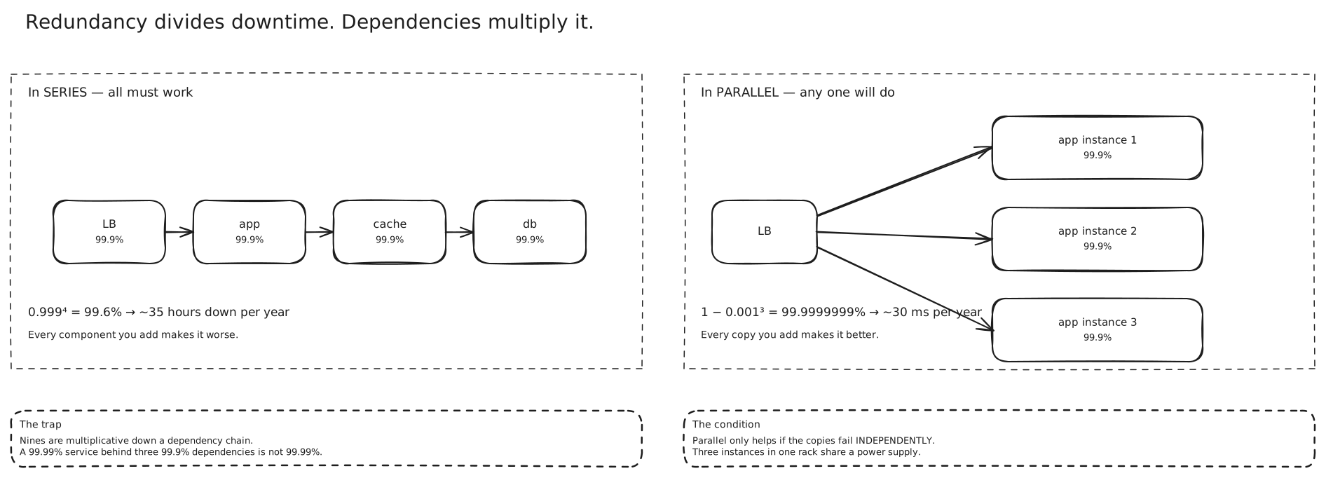
It isn’t 99.9%. Components in series multiply:
0.999 × 0.999 × 0.999 = 0.99700 → 99.70%, about 26 hours per yearYou built three three-nines components and shipped a two-nines feature. Add the two dependencies that any real checkout has — a payment gateway and a fraud check — and it gets worse:
0.999^5 = 0.99501 → 99.50%, about 44 hours per yearIt’s usually not that uniform in practice. A managed load balancer might be 99.99%, your database 99.95%, your own services 99.9%. Multiply them out and you land around 99.64%, roughly 31 hours a year. The shape of the result is the same either way: the chain is always worse than its worst link, and it gets worse with every link you add.
This is the single most useful thing on this page for an interview, because it reframes “should we extract this into a microservice?” as an availability question. Every synchronous call you add to a request path is a multiplication. It’s also the argument for making a dependency asynchronous: if the fraud check goes on a queue and checkout doesn’t block on it, it drops out of the product entirely. → Message Queues
Redundancy divides instead of multiplying
Two app servers behind the load balancer, either one able to serve the request. Now the pair is only down when both are down. The probability of both failing is the product of their individual failure probabilities:
A = 1 − (1 − 0.999) × (1 − 0.999)
  = 1 − 0.001 × 0.001
  = 0.999999        →  99.9999%,  5.26 minutes per year
Two three-nines boxes became a six-nines pair. Add a third and the formula says nine nines — about a third of a second per year.
Put the two rules together and a real architecture is a series of parallel groups. Redundant load balancers in front of redundant app servers in front of a replicated database:
0.999999 × 0.999999 × 0.999999 = 0.999997 → about 1.6 minutes per yearNinety seconds of downtime a year. If you have ever operated anything, you know that’s nonsense.
Why the arithmetic lies
The parallel formula has an assumption baked into it that nobody says out loud: failures are independent. Multiplying 0.001 × 0.001 is only valid if the second server’s chance of dying is unaffected by the first one dying. In production it is spectacularly affected.
Your two app servers are running the same binary, so the bad deploy kills both. They read the same config, so the bad config kills both. They’re in the same rack on the same power feed in the same availability zone, so the power event kills both. They talk to the same database, so when it gets slow they both fill their thread pools and stop responding. And when the first one dies, the second one inherits all its traffic — which is exactly the condition most likely to kill it too.
The other thing the formula hides is that failover isn’t free or instant. A database replica only helps if something detects the primary is dead and promotes the replica, and that takes time — commonly minutes, not milliseconds. So the honest availability of a primary/replica pair is closer to “the availability of the pair, times the probability failover actually works, minus the failover window.” Which is why the number you should quote is one you’ve measured in a game day, not one you computed. → Disaster Recovery
Patterns for spending money on redundancy
Active-active. Every replica takes live traffic. There’s no failover step, because there’s nothing to fail over to — you just stop sending traffic to the dead one. Fastest recovery, most expensive, and it forces you to solve concurrent writes if the redundant thing is stateful.
Active-passive. One serves, one waits. The standby can be hot (running, fully sized, ready now), warm (running, scaled down) or cold (not running). The colder it is, the cheaper it is and the longer your MTTR. That whole spectrum is the subject of Disaster Recovery.
N+1 and N+2. Size for the load you need plus one spare, or plus two. N+1 survives one failure. N+2 survives one failure while a node is out for maintenance, which is the case that actually bites you, because maintenance windows are exactly when you’re least redundant.
Quorum. Instead of one primary, a group of an odd number that votes. Survives the loss of a minority and, crucially, avoids two nodes both believing they’re the primary. → Clustering
One sharp point: whatever you put in front of a redundant group is now a series component. A load balancer fronting ten app servers is a single point of failure for all ten, which is why load balancers are themselves deployed in pairs with a floating address or with DNS/anycast in front. → Load Balancing
Available, reliable and durable are three different promises
These get used interchangeably and they aren’t the same claim.
Availability asks: is it responding right now? Reliability asks: does it do the right thing, consistently, over time? A service that crashes and restarts every thirty seconds but recovers in one millisecond is wildly available and completely unreliable. A batch job that runs once a night and is always correct is highly reliable and, by an uptime measure, almost never available.
The relationship is one-directional. If a system is reliable it will also be available; being available says nothing about whether it’s reliable.
And the failure mode that catches teams out: a service returning HTTP 200 with wrong or empty data counts as “available” under a naive health check, and users experience it as an outage. If your availability metric can’t tell the difference between a correct answer and a confident wrong one, it isn’t measuring availability. That’s why good measurement is defined in terms of successful user-visible operations, which is the whole argument of SLA SLO SLI.
Durability is the third one: once you accept a write, does the data still exist later? A system can be unavailable for an hour and perfectly durable, or available all day and quietly losing writes. Storage systems publish availability and durability as separate figures for exactly this reason.
Availability in CAP means something stricter
Careful here, because the word gets reused. In CAP Theorem, availability is a formal property: during a network partition, every request to a non-failing node returns a non-error response. It’s binary, and it’s a statement about behaviour under partition, not a percentage over a year.
A system can be “AP” in the CAP sense and still have terrible operational uptime, and a “CP” system that rejects writes during a partition may still report 99.99% availability for the year, because partitions are rare. The two ideas are related in spirit and unrelated in measurement. Say the right one in an interview. → PACELC Theorem
Your DR plan is a line item in your availability budget
Here’s the arithmetic that connects the two notes. Suppose you lose a whole region once every three years, and your recovery plan takes six hours. Averaged out, that’s two hours of downtime per year from that one scenario.
A three-nines budget is 8.76 hours a year in total. So one rare regional failure, handled by a plan you consider reasonable, has already eaten roughly a quarter of your annual budget before a single bug ships. Shrink the recovery to thirty minutes and it costs you ten minutes a year instead.
That’s the honest way to decide how much to spend on a standby environment: not “do we want a DR plan,” but “what does our RTO cost us in nines?” → Disaster Recovery
Where this shows up
- Cloud SLAs are quoted per component and compose the way this note describes — a managed load balancer at 99.99%, a multi-AZ database at 99.95% and your own service at 99.9% produce a number lower than any of them.
- Multi-AZ deployment is a direct application of the independence caveat: the whole product is “these replicas do not share power, cooling or network.”
- Staged rollouts and canaries exist because a bad deploy is the most correlated failure there is, and it defeats every redundancy you paid for.
- Chubby, Google’s lock service, is deliberately taken down when it exceeds its availability target, so that dependent teams don’t build on an uptime that isn’t promised.
In an interview
Bring it up the moment you draw a second synchronous dependency on the request path — say “note that these multiply, so this path can’t be better than 99.7%” and you’ve shown the arithmetic without being asked.
Expect to be pushed on redundancy. The naive answer is “add a replica”; the good answer names the failure domain the replica sits in and admits the failover window. If you claim five nines, be ready to explain what automation achieves a one-minute-per-week MTTR.
The most common mistake is listing “highly available” as a non-functional requirement with no number attached. Pick a target, justify it from the business cost of downtime, and then check your own architecture’s serial chain against it. The second most common mistake is conflating CAP-availability with uptime.
Seen in
- Uber · Requirements and Estimation — the trap of answering “non-functional requirements?” with “highly available, strongly consistent, low latency”, and why different parts of one system get different guarantees
Related
SLA SLO SLI · Disaster Recovery · CAP Theorem · Scalability · Clustering · Load Balancing · Replication and Read Consistency · Circuit Breakers