Stage 01 · Foundations
Databases and DBMS
When you draw a cylinder on a whiteboard and call it “the database”, you’ve just hidden five or six independent subsystems inside it. Knowing which one you’re leaning on — and which one is about to break — is what makes the rest of the discussion precise.
The fastest way to see what those subsystems are is to try building without them.
The world’s simplest database
Let’s store orders for an online store. Here is a complete, working database in two lines of shell:
db_set () { echo "$1,$2" >> orders.db; }
db_get () { grep "^$1," orders.db | tail -n 1 | cut -d, -f2-; }$ db_set 41234 '{"user":"ana","total":38.50,"status":"paid"}'
$ db_get 41234
{"user":"ana","total":38.50,"status":"paid"}Don’t dismiss this. The write path is genuinely excellent — an append to the end of a file is a sequential write, which is the fastest thing a disk does, and real storage engines do exactly this at their core. Updating a record appends a new line and tail -n 1 picks the newest, so writes never have to find anything first.
The read path is where it falls over. grep scans the entire file.
At a thousand orders that’s invisible. At ten million orders the file is a few gigabytes, and reading a gigabyte sequentially from disk costs about 20 ms per megabyte, so a single lookup takes tens of seconds. Every read costs more as the database grows, which is the one property you can never accept.
Fix one: stop scanning
The fix is to keep a second structure whose only job is to answer “where is order 41234?” — a map from key to byte offset in the file. Now a read is one lookup and one seek instead of a full scan.
That’s an index, and it’s the first subsystem. It also introduces the first real trade in databases: every index you add makes reads faster and writes slower, because the write now has to update the table and every index over it. An index is never free, and there’s a lot more to say about the shapes they come in. → Database Indexes
Fix two: the process dies
Now kill the process mid-write.
Two bad things happened. The in-memory index is gone, so you have to rebuild it by scanning the whole file again. Worse, the last echo may have written half a line — the disk was happy to flush 30 bytes of a 60-byte record — so the file itself is now corrupt at the tail.
The standard fix is a write-ahead log. The rule is one sentence: never change a data page on disk until a record describing that change has been flushed to the log. Postgres states it plainly — data pages don’t need to be flushed on every commit, “because we know that in the event of a crash we will be able to recover the database using the log.”
On restart, the engine reads the log from the last checkpoint forward and re-applies everything it finds. A half-written log record fails its checksum and is discarded along with everything after it, so the database comes back at a consistent point, having lost only transactions that were never acknowledged.
The subtle part is that the WAL makes things faster, not slower. The log is written sequentially, so an fsync of the log is cheap, whereas flushing the actual modified pages means random writes scattered across the file. And because many transactions land in the same log segment, a single fsync can commit a whole batch of them at once — group commit. You turned a lot of expensive random durability into one cheap sequential one.
Fix three: every read still hits the disk
Reads are correct now but they still go to storage. From the latency ladder, memory is around 100 ns and a random 4 KB SSD read is around 150,000 ns — a factor of a thousand and a half. → Storage
So the engine keeps its own cache of pages in memory: the buffer pool. Postgres calls it shared_buffers and suggests roughly 25% of system RAM as a starting point on a dedicated server, noting that going past 40% tends to be counterproductive because the OS page cache is doing work too. MySQL/InnoDB calls it the buffer pool and generally gets given far more.
The buffer pool and the WAL are designed to work together, and this is the pairing worth remembering. A write modifies a page in memory and appends to the log. The page is now “dirty” and sits there, possibly for minutes. Durability came from the log; the expensive page write got deferred and will eventually be batched with other changes to the same page. Commit at the speed of a sequential append, with the read performance of an in-memory cache. That combination is most of why a real database beats a file.
It also tells you the single most important capacity question about a database: does the working set fit in the buffer pool? A database whose hot pages fit in RAM and one whose hot pages don’t are two different systems running the same code.
Fix four: two clients at once
Two order-processing workers both read order 41234, both decide it’s unpaid, and both charge the card.
Preventing that is the transaction manager, and it’s doing two separate jobs: making a group of changes atomic (all or nothing, using the same log), and deciding what concurrent transactions are allowed to see of each other. The second job is the one with all the subtlety in it, and it has its own note. → Transactions and Isolation, ACID and BASE
Fix five: a question you didn’t plan for
Finally, someone asks for “the total value of unpaid orders placed in the last week, by country.”
Our shell database can’t answer that at all. Even with the index, the index only answers one question — lookup by order id. Answering a new question means writing new traversal code by hand.
A query planner is the subsystem that removes that work. You declare what you want and it decides how: which index to use or whether to ignore them all, what order to join tables in, which join algorithm to run.
Postgres’s optimiser builds candidate “paths” for each relation and costs them. A sequential scan is always generated as a baseline. An index scan is generated only if an index matches the query’s restriction and the operator class supports the operator. Then it picks whichever path is cheapest — which is why the same query gets a different plan as the table grows, and why it goes back to a sequential scan when your WHERE clause matches 40% of the rows. For joins it chooses between nested loop, merge join and hash join, and it searches join orderings near-exhaustively until the number of relations exceeds geqo_threshold, at which point it switches to a genetic algorithm because the search space has stopped being tractable.
That’s the whole point of declarative querying: the plan is chosen at run time, against current statistics, rather than baked into your code at the moment you wrote it. → SQL Databases
So that’s what you’re buying
Walk back up the chain and the “database” cylinder has resolved into named parts:
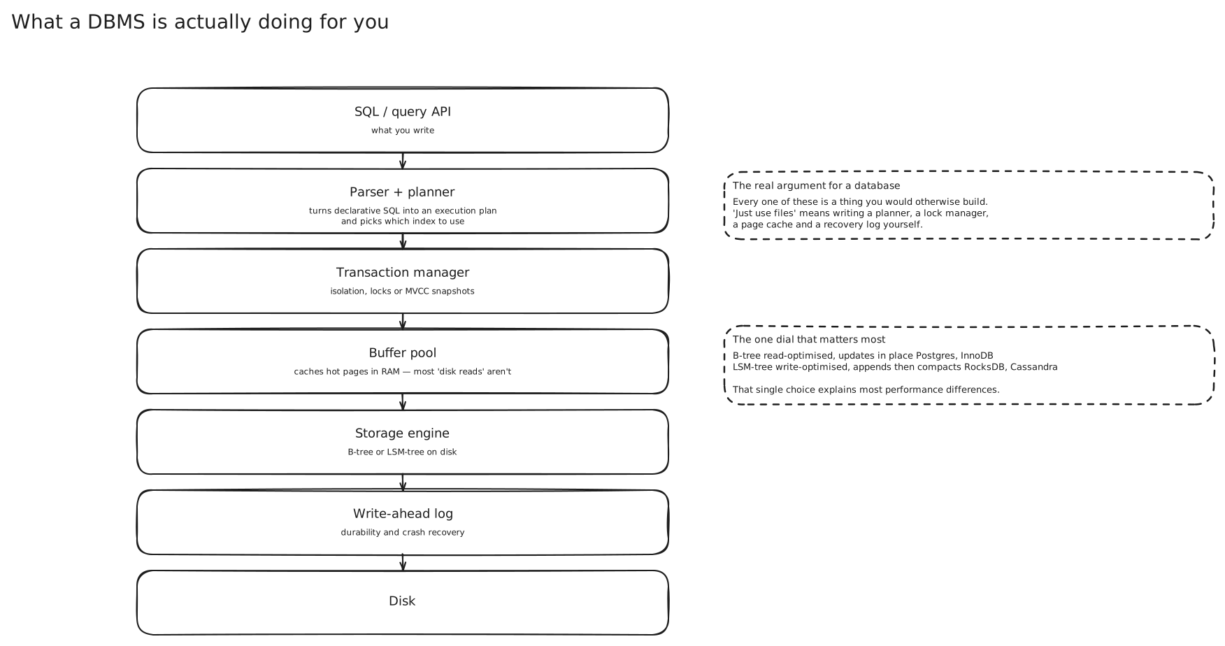
Two of those boxes — the planner and the storage engine — are where almost every interesting design difference between databases lives. The rest is broadly the same everywhere.
Two shapes of workload
Before comparing storage engines it’s worth splitting the workloads, because they want opposite things.
Our online store has to do two kinds of work. The first is “charge this customer, mark this order paid, decrement this stock count.” Small reads and writes, always by primary key, thousands per second, each one has to come back in milliseconds because a human is waiting. That’s OLTP — online transaction processing.
The second is “revenue by product category by week for the last two years.” One query, touching every order ever placed, reading three columns out of thirty, returning forty rows. Nobody runs it more than a few times a day and nobody minds if it takes ten seconds. That’s OLAP — online analytical processing.
The uncomfortable part is that running the second on the same machine as the first is how you take down the first. That analytical query scans hundreds of gigabytes, which evicts every hot OLTP page from the buffer pool, and now your checkout latency is a disk read per row. This is the usual reason a company builds a separate warehouse — not because the warehouse is faster at analytics, but because it keeps analytics away from the transaction path. → CQRS, Replication and Read Consistency
Row storage versus column storage
Here’s why the warehouse is also genuinely faster. It comes down to what the unit of I/O is.
Disk reads happen in pages — 8 KB in Postgres, and the block layer beneath reads 4 KB at a minimum. You can’t read a field; you read the page it’s on.
A row-oriented engine stores each record’s fields next to each other:
row store, one 8 KB page:
[id|user|cat|price|ts|addr|phone|notes…][id|user|cat|price|ts|addr|phone|notes…]…
  ^^^     ^^^  ^^^^^
  the three columns you asked for, buried in ~400 bytes of row you didn't
So SELECT category, SUM(price) FROM orders WHERE created_at > ... drags every shipping address, phone number and note off disk, because they share a page with the columns you wanted. If your rows are 400 bytes and you need 30 bytes of them, you just wasted 92% of your disk bandwidth.
A column-oriented engine stores each column contiguously instead:
column store:
category:  [home][home][toys][toys][toys][books]…   ← read only this
price:     [38.50][12.00][9.99][42.10][7.25]…       ← and this
address:   [...]                                     ← never touched
Now the query reads exactly the two columns it named. That alone is the 10× or more, and then compression multiplies it: a column holds one data type with heavily repeated values, so run-length encoding turns a million "home" entries into a count and a string. ClickHouse’s own introduction puts numbers on the result — a query over 100 million rows finishing in 92 ms, “approximately over 1 billion rows per second or just under 7 GB of data transferred per second.”
The reason OLTP databases don’t do this is the mirror image. Fetching one whole order from a column store means one read per column and then stitching them back together, and inserting one order means touching thirty separate column files. Columns are wonderful for reading a few fields of everything and terrible for reading everything of one row.
That’s the whole story: row stores optimise for “all of one record”, column stores optimise for “one field of all records.” Postgres, MySQL and Oracle are row stores. Redshift, BigQuery, Snowflake, ClickHouse and Parquet files are column stores. → SQL vs NoSQL
B-tree versus LSM-tree
Now the storage engine choice that actually comes up, and the one worth being able to reason about out loud.
The B-tree updates in place
A B-tree keeps keys sorted in fixed-size pages, with internal pages holding pointers to child pages. Postgres and InnoDB both use pages of about 8 KB and 16 KB respectively, and the fanout is high enough that even a billion-row table is only about four levels deep. A lookup is therefore three or four page reads, and the top levels are always in the buffer pool, so in practice it’s one disk read.
Updating a row means finding its leaf page, changing the bytes in that page, and writing the page back. In place. That’s the defining property, and it has two consequences.
The good one: reads are cheap and predictable. One key lives in exactly one place. Range scans walk the leaves in order. The planner can cost it accurately because the depth barely varies.
The bad one shows up under a write-heavy load. Insert a million records with random keys — order ids, UUIDs, user ids — and each insert lands on a different leaf page. To change 50 bytes you dirty and eventually rewrite an entire 8 KB page, and you’d already written those 50 bytes to the WAL, so the same data hits the disk twice. On top of that, pages fill up and split, which fragments the file and makes subsequent range scans less sequential than they look.
This is write amplification: bytes actually written to storage divided by bytes your application handed over. For a B-tree taking random-key inserts it is comfortably in the tens.
The LSM-tree buffers and merges
An LSM-tree — log-structured merge-tree — refuses to do random writes at all.
Writes land in a sorted in-memory structure called the memtable, plus one sequential WAL append for durability. Nothing touches the main data files. When the memtable fills, it’s flushed out whole as an immutable sorted file (an SSTable) — one big sequential write. A background process, compaction, merges those files together over time, discarding overwritten and deleted keys as it goes. RocksDB organises them in levels, with the newest data in L0 and older data pushed down toward Lmax.
Look at what that did to the write path. A thousand random-key inserts no longer produce a thousand scattered page rewrites. They produce one memtable insert each, and eventually one sequential file. The foreground write cost collapsed.
What the fix costs you
Reads got harder. A key could be in the memtable, or in any L0 file, or in L1, or below. Worst case you check them all — that’s read amplification. The standard mitigations are a bloom filter per SSTable, so a file that definitely doesn’t contain the key is skipped without a disk read, and level compaction, which guarantees non-overlapping key ranges below L0 so at most one file per level can match. Range scans are worse off than point reads, because you have to merge-iterate across every level at once and can’t bloom-filter your way out of it.
Space got harder. Until compaction runs, an overwritten key exists in several files and a deleted key exists as a tombstone. That’s space amplification.
And write amplification didn’t disappear — it moved. Compaction rewrites the same data every time it’s merged down a level, so the total bytes written can still be large. What changed is when. B-tree write amplification is paid in the foreground, on the transaction that’s waiting. LSM write amplification is paid in the background, by a compaction thread, where it costs throughput and disk wear instead of latency. That’s the trade in one sentence, and it’s the one to say out loud.
You can’t escape this triangle, only pick a corner. That’s the RUM conjecture: bound any two of read overhead, update overhead and memory (space) overhead, and you’ve set a lower bound on the third. RocksDB’s own documentation is refreshingly blunt about it — level compaction “optimizes disk footprint versus logical database size (space amplification)”, universal compaction “optimizes total bytes written to disk (write amplification)” and consequently has “lower write-amplification but higher space- and read-amplification than Level Style.”
| B-tree (Postgres, InnoDB) | LSM-tree (RocksDB, Cassandra) | |
|---|---|---|
| Write path | random page updates in place | sequential appends + background merge |
| Write amplification | high, paid in the foreground | high, paid by compaction threads |
| Point read | ~1 disk read, very predictable | memtable + bloom filters + 1 file per level |
| Range scan | walk the leaves, naturally sequential | merge-iterate across all levels |
| Space | fragmentation, partly-empty pages | tombstones and duplicates until compaction |
| Latency shape | flat | mostly flat, with compaction-induced spikes |
Who uses which, and why it isn’t the SQL/NoSQL line
B-tree: PostgreSQL, MySQL’s InnoDB, SQL Server, SQLite, MongoDB’s WiredTiger, and essentially every general-purpose index. LSM: RocksDB, LevelDB, Cassandra, ScyllaDB, HBase, and the storage layer under a great many message and metrics systems.
The tempting shortcut is “SQL means B-tree, NoSQL means LSM.” It isn’t true and saying so is a nice signal of depth. MyRocks is MySQL running on RocksDB — a fully relational, transactional SQL database on an LSM engine — and organisations move to it precisely to cut write amplification and gain compression on write-heavy tables. The storage engine is a property of the workload, not of the query language. → SQL vs NoSQL
Where this shows up
- Choosing a warehouse. Anything ending in “…by day, by region, for the last year” wants columnar storage — BigQuery, Redshift, Snowflake, ClickHouse — fed from the transactional store, not run against it.
- Metrics and time-series ingestion. Millions of appends per second with reads almost always by
(series, time range)is the canonical LSM workload, which is why InfluxDB, Cassandra and RocksDB-backed systems dominate there. - Tuning a struggling Postgres. “Is the working set bigger than
shared_buffers?” and “how many indexes is this write updating?” are the first two questions, and both come straight out of the subsystem map. → SQL Databases - Replication and backups. Both are built on the WAL: a replica is a process replaying the primary’s log, and point-in-time recovery is replaying an archived one. → Replication and Read Consistency, Disaster Recovery
In an interview
Bring this up when someone challenges your database choice. Answering at the level of “Cassandra is good at writes” is weak; answering “it’s an LSM, so random-key writes become sequential appends” is the same answer with a mechanism behind it.
Expect to be pushed on the cost. If you claim LSM write performance, be ready for “so what gets worse?” — read amplification, space amplification, and compaction spikes in the tail latency.
The OLTP/OLAP split is worth volunteering unprompted the moment analytics appear in the requirements. Saying “I’d keep that off the transactional primary so a table scan can’t evict the checkout path’s hot pages” is a concrete reason, not a slogan.
The most common mistake is talking about databases as monoliths — “Postgres can’t scale” — when the real statement is always about one subsystem: the write path, the buffer pool, the connection model, or maintenance. Name the part. → Scalability
Seen in
- 12 - How Uber Actually Does It — Docstore moved its storage engine from InnoDB to MyRocks in 2019 for exactly the reasons above: write amplification and compression, with the SQL layer unchanged.
Related
Database Indexes · SQL Databases · NoSQL Databases · SQL vs NoSQL · Transactions and Isolation · Storage · Normalization and Denormalization · ACID and BASE
Sources
- PostgreSQL — Write-Ahead Logging (WAL)
- PostgreSQL — Planner/Optimizer
- PostgreSQL — Resource Consumption (
shared_buffers) - RocksDB Wiki — RocksDB Overview
- ClickHouse — What is ClickHouse? (column-oriented storage)
- Alex Petrov — Algorithms Behind Modern Storage Systems (ACM Queue)
- Hello Interview — Database Indexing deep dive