Stage 02 · The database core
Database Indexes
An index is a second copy of part of your data, arranged so the database can find rows without looking at all of them. Everything interesting about indexes falls out of one fact: you buy that copy once, and you pay for it on every write for the rest of the table’s life.
This note is about indexes on one machine — one table, one disk, one tree. Once the table is split across shards, “just add an index” stops being a one-line decision and becomes an architectural one, and that’s a different note: Secondary Indexes at Scale. Get the single-node story straight first, because the sharded version only makes sense as a thing that breaks it.
The query that was fine last quarter
You’re running the orders table for an online store.
CREATE TABLE orders (
  order_id     bigint PRIMARY KEY,
  customer_id  bigint NOT NULL,
  email        text   NOT NULL,
  status       text   NOT NULL,
  total_cents  int    NOT NULL,
  created_at   timestamptz NOT NULL
);
Support has a screen that looks up an order by the customer’s email. The query is the obvious one:
SELECT * FROM orders WHERE email = 'ada@example.com';With 5,000 rows this is instant, and it’s instant for a boring reason — the whole table fits in memory and the database reads all of it. That’s a sequential scan: start at the first row, check the predicate, move on, stop at the end. Cost is linear in table size. Nobody notices linear when the constant is small.
Two years later the table has 80 million rows. The same query now reads 80 million rows to return one. Ask Postgres what it’s doing and it tells you plainly:
EXPLAIN SELECT * FROM orders WHERE email = 'ada@example.com';

 Seq Scan on orders  (cost=0.00..1834210.00 rows=1 width=96)
   Filter: (email = 'ada@example.com'::text)
Read that as: I will start at cost 0, finish at cost 1.8 million, and hand you back 1 row. The database is doing 80 million units of work to produce one unit of answer. That ratio is the whole problem.
So what do we actually want? We want what a phone book gives you. Not “read every name until you hit Hopper” but “the names are in order, so jump.”
Try the obvious thing: keep a sorted copy
Make a second structure. It holds just (email, pointer-to-row), sorted by email. Now finding Ada is a binary search: 80 million rows is about 27 halvings. Twenty-seven comparisons instead of eighty million.
That works beautifully for reads and dies immediately on writes. A sorted array has to stay sorted. Insert an order for aaron@example.com and every entry after it shifts one slot down. One insert, tens of millions of bytes moved. You’ve made reads 3-million-times faster and writes unusable.
And there’s a second problem you only see once you remember this lives on disk. Binary search jumps around: position 40M, then 20M, then 30M. Each jump is a separate random read. Disks — even SSDs — are much happier reading a contiguous block than chasing pointers. A structure that’s optimal for in-memory binary search is not automatically optimal for disk.
So we need a sorted structure that tolerates inserts and is shaped like disk pages. That’s a B-tree.
B-trees: the default for a reason
A B-tree (in practice, a B+tree) is a shallow, wide, balanced tree. Two design decisions make it the right shape:
One node = one disk page. Postgres’s default block size is 8 kB, and an index node is one block. So a node isn’t a two-child thing like a binary tree — it holds as many keys as fit in 8 kB. If a key plus its pointer runs around 20 bytes, that’s roughly 400 entries per node. (Wide text keys give you fewer; a bigint key gives you more. The point is the order of magnitude, not the number.)
All leaves sit at the same depth, and the tree rebalances by splitting nodes rather than shifting everything. An insert touches one leaf; if it’s full, the leaf splits and one key gets pushed up. Occasionally that cascades. Usually it doesn’t.
Put those together and the depth arithmetic is startling. With a fanout of ~400: one level addresses 400 entries, two levels 160,000, three levels 64 million, four levels 25 billion. Four page reads gets you to any row in a table with billions of rows — and the top two levels are almost certainly already cached, so in practice it’s one or two actual disk reads.
Here’s the shape. Look at the bottom row: the leaves are chained together as well as hanging off their parents.
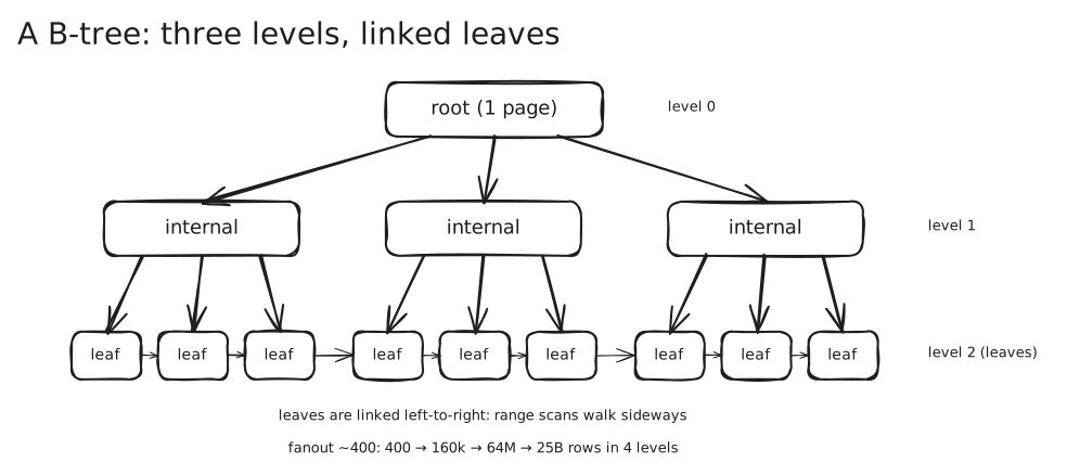
That last line is the other reason B-trees win. The leaves form a sorted linked list, so once you’ve found the first matching entry you can walk sideways. WHERE created_at BETWEEN '2026-01-01' AND '2026-02-01' is one descent plus a sequential walk. ORDER BY created_at is free — you’re already reading in order.
This is why B-tree is the default index type everywhere. It handles equality, ranges, sorting, IS NULL, and anchored prefix matches like LIKE 'ada%', all with the same structure. Postgres’s list of B-tree operators is exactly that set: < <= = >= >, plus BETWEEN, IN, IS NULL, and pattern matches anchored at the start of the string.
Now the plan changes:
EXPLAIN SELECT * FROM orders WHERE email = 'ada@example.com';

 Index Scan using orders_email_idx on orders  (cost=0.57..8.59 rows=1 width=96)
   Index Cond: (email = 'ada@example.com'::text)
1.8 million down to 8.6.
Reading the plan, because guessing is worse
You should never have to argue about whether an index is being used. EXPLAIN tells you, and it’s the single most useful debugging tool in this entire note.
Plain EXPLAIN shows the planner’s estimate: cost=startup..total, rows (how many it expects), width (average bytes per row). Costs are in arbitrary units — conventionally scaled to disk page fetches — so they’re only meaningful relative to each other. EXPLAIN ANALYZE actually runs the query and adds actual time=startup..total, rows, and loops.
The node types you need to recognise:
- Seq Scan — reading the whole table. Fine for small tables and for queries that genuinely want most of the rows. Alarming on a big table with a selective predicate.
- Index Scan — descend the tree, then fetch each matching row from the table itself. Two structures touched per row.
- Bitmap Heap Scan (with a Bitmap Index Scan under it) — the index found lots of matches, so rather than chasing them one at a time in index order, the database builds a bitmap of which pages it needs and reads them in physical order. This is the planner deciding that random I/O is worse than a bit of extra sequential I/O.
- Index Only Scan — answered entirely from the index. The table was never touched. More on this below.
Also watch loops. A node showing actual time=0.003..0.003 ... loops=10000 took 30 ms total, not 0.003 ms. That’s how a nested loop join quietly becomes the whole query.
Hash indexes: faster at exactly one thing
If all you ever do is equality, the tree descent is wasted motion. A hash index hashes the key straight to a bucket — O(1), no comparisons, no depth.
CREATE INDEX orders_email_hash ON orders USING HASH (email);Postgres supports exactly one operator on a hash index: =. That’s the entire trade. No ranges, no ORDER BY, no LIKE 'ada%', no using it as the leading column of a sort. The moment a new query needs a range you’re adding a B-tree anyway, and now you have two indexes on the same column.
The honest conclusion is that hash indexes are rarely worth it on disk-based databases — the B-tree is already 1–2 reads and it does everything else too. Where hashing genuinely wins is in memory: Redis hash tables, an in-process cache, the hash table built on the fly by a Hash Join. Know it exists, know why the default isn’t it.
Composite indexes and the leftmost-prefix rule
Support’s next screen is “this customer’s orders, newest first”:
SELECT * FROM orders WHERE customer_id = 4711 ORDER BY created_at DESC LIMIT 20;You could index customer_id and created_at separately, but then the database finds all of customer 4711’s orders — possibly thousands — and sorts them. Instead, index both in one tree:
CREATE INDEX ON orders (customer_id, created_at);Entries are sorted by customer_id first, and within each customer, by created_at. So the query is one descent to the start of customer 4711, then a walk of 20 leaf entries. No sort at all.
Column order is the whole ballgame. The Postgres docs state the rule precisely:
“Equality constraints on leading columns, plus any inequality constraints on the first column that does not have an equality constraint, will always be used to limit the portion of the index that is scanned.”
Unpacked, against (customer_id, created_at):
WHERE customer_id = 4711— great. Leading column, equality.WHERE customer_id = 4711 AND created_at > '2026-01-01'— ideal. Equality on the first, range on the second.WHERE created_at > '2026-01-01'— the index can’t narrow the scan. The tree is sorted by customer first, so January’s orders are scattered across the entire index, once per customer.
That last case is the leftmost-prefix rule people actually get bitten by. An index on (a, b, c) serves queries on a, on (a, b), and on (a, b, c). It does not serve a query on b alone any better than a full scan of the index would.
Modern Postgres softens this with skip scan: if the leading column has few distinct values, the planner can rewrite WHERE y = 7700 into repeated searches, one per distinct x. That’s a genuine optimisation, and it’s also a trap in an interview — it works because there are few distinct leading values. With 50 million distinct customer_ids it saves you nothing.
The other rule worth knowing: don’t get carried away. Postgres allows up to 32 columns in an index, and then says in the same breath that “indexes with more than three columns are unlikely to be helpful unless the usage of the table is extremely stylized.” Every extra column makes the index bigger and the writes more expensive, in exchange for helping a narrower and narrower set of queries.
Covering indexes, and the heap fetch you forgot about
Look again at the Index Scan plan. It descends the tree, finds the entry, and then — because the index only stores the indexed columns plus a row pointer — it goes and fetches the actual row. That second step is the heap fetch, and for a query returning many rows it’s the dominant cost, because those rows are scattered anywhere across the table.
Now consider a query that doesn’t need the whole row:
SELECT order_id, total_cents FROM orders WHERE customer_id = 4711;If the index already contains customer_id, order_id and total_cents, the heap has nothing left to give. Postgres can skip it entirely — an index-only scan.
CREATE INDEX ON orders (customer_id) INCLUDE (order_id, total_cents);INCLUDE adds payload columns that aren’t part of the search key. They’re along for the ride: the docs note the included column “is merely stored in the index and is not interpreted by the index machinery,” so it doesn’t even need a type the index knows how to compare. And on a unique index, uniqueness applies only to the key columns, not the included ones — which is occasionally exactly what you want.
There’s a subtlety that trips people up, and it’s a nice thing to know. An index entry doesn’t record whether its row is visible to your transaction — that lives with the row. So how can an index-only scan skip the heap without risking showing you a deleted row? Postgres keeps a visibility map: one bit per table page saying “every row on this page is visible to everyone.” The scan checks that bit first; if it’s set, no heap fetch. The map is, in the docs’ words, “four orders of magnitude smaller than the heap it describes.”
The practical consequence is that index-only scans depend on VACUUM having run — one of the four documented reasons VACUUM exists is to update the visibility map. A table under heavy write load with vacuum falling behind will quietly stop getting index-only scans and nobody will know why.
Clustered vs secondary: where the row actually lives
So far the index has been a side structure pointing at a table. That’s Postgres’s model: a heap of rows in no particular order, and every index — including the primary key’s — is a separate tree holding pointers into it. Every index is a secondary index.
MySQL’s InnoDB does it differently, and the difference matters.
“Each InnoDB table has a special index called the clustered index that stores row data. Typically, the clustered index is synonymous with the primary key.”
The primary key index is the table. The leaves don’t hold pointers to rows — they hold the rows. Which means a primary key lookup is one descent and you’re done, no heap fetch, ever. “Accessing a row through the clustered index is fast because the index search leads directly to the page that contains the row data.”
The cost shows up in secondary indexes. In InnoDB, “each record in a secondary index contains the primary key columns for the row, as well as the columns specified for the secondary index.” There’s no direct row pointer, because rows move when the clustered index rebalances. So a secondary index lookup is two tree descents: find the primary key in the secondary index, then find the row in the clustered index.
Two consequences fall out of this immediately:
Keep the primary key short. Every secondary index carries a full copy of it in every entry. The docs say it outright: “if the primary key is long, the secondary indexes use more space.” A 36-character UUID string as your PK is duplicated into every entry of every other index on the table.
Insert order matters on a clustered index. Rows are stored in primary-key order, so a monotonically increasing key appends to the end of the structure. A random key inserts into the middle of a random page, which fills pages unevenly and causes splits. This is the actual mechanism behind “don’t use random UUIDs as an InnoDB primary key” — and it’s also why time-ordered UUID variants exist.
If nothing else, remember this when someone asks why the same schema performs differently on Postgres and MySQL. It’s often not the query. It’s the storage layout.
Partial indexes: index the rows you actually query
Most of the orders table is finished business. The open orders — the ones the fulfilment system polls for every few seconds — are a tiny fraction.
An index on status covers all 80 million rows so that you can find the 40,000 you care about. A partial index covers only the rows matching a predicate:
CREATE INDEX orders_open_idx ON orders (created_at) WHERE status = 'OPEN';Smaller tree, fewer levels, and — the part people forget — cheaper writes. A row that doesn’t match the predicate doesn’t get an index entry at all, so the other 79,960,000 orders cost nothing to maintain here.
The Postgres docs give three uses, and the third is the interesting one. Beyond excluding common values and excluding uninteresting ones, a partial index can enforce uniqueness over a subset:
CREATE UNIQUE INDEX ON orders (customer_id) WHERE status = 'OPEN';“At most one open order per customer,” enforced by the database, atomically, in one statement. No application-level check, no race. It’s the cheapest correct answer to a whole class of “can this happen twice?” problems — and knowing it is the setup for understanding why the sharded version is so much harder. → Secondary Indexes at Scale
What every index costs you
Here’s the part that separates a candidate who has run a database from one who has read about them. Indexes are not free reads. They are a tax on writes, paid forever.
Insert one row into orders with five indexes on it, and the database does six writes: the row, plus an entry in each of the five trees. Each of those may split a page. Each is a separate write-ahead-log record. Your single INSERT is a six-fold write amplification.
UPDATE is worse in a subtle way. Updating a column that no index covers might touch only the row. Updating an indexed column means deleting the old index entry and inserting a new one — in Postgres, where an update writes a whole new row version, that can mean re-inserting into every index on the table.
Then there’s space. An index on a wide text column can approach the size of the table itself. Indexes compete with your data for page cache. An index nobody uses still gets maintained on every write, still gets vacuumed, and still evicts hot data from memory.
So the discipline is: find the unused ones and drop them.
SELECT relname, indexrelname, idx_scan
FROM pg_stat_user_indexes
WHERE idx_scan = 0
ORDER BY pg_relation_size(indexrelid) DESC;
Zero scans since the stats were reset means nothing has ever used it. That’s pure cost.
When a B-tree is the wrong shape (1): inverted indexes
Support now wants to search order notes for the word “refund”.
SELECT * FROM orders WHERE notes LIKE '%refund%';A B-tree on notes is useless here, and the reason is structural, not a missing optimisation. The tree is sorted by the whole string from the left. LIKE 'refund%' is a prefix, so it’s a range and the tree handles it. LIKE '%refund%' says “the word is somewhere in the middle,” and there is no contiguous range of the sorted order that contains all such strings.
The fix is to change what gets indexed. Instead of one entry per document keyed by the whole document, make one entry per term, and let its value be the list of documents containing it. That’s an inverted index — inverted because the mapping runs from content to document rather than document to content.
  "refund"  ->  [ 17, 402, 9981, 10334, ... ]
  "damaged" ->  [ 402, 6650, ... ]
  "late"    ->  [ 17, 88, 9981, ... ]
Now “documents containing refund AND damaged” is an intersection of two sorted integer lists, which is fast and streams. Ranking (which of these is most relevant?) is a separate layer on top, using term frequency and how rare the term is across the corpus.
Postgres ships this as GIN: “GIN indexes are ‘inverted indexes’ which are appropriate for data values that contain multiple component values, such as arrays. An inverted index contains a separate entry for each component value.” Which is why the same index type serves full-text search, JSONB containment, and array membership — they’re all “does this composite value contain this component?”
CREATE INDEX orders_notes_idx ON orders USING GIN (to_tsvector('english', notes));Dedicated search engines — Elasticsearch, anything on Lucene — are inverted indexes with a great deal of machinery around them: analysers, stemming, relevance scoring, distribution. The core data structure is the same one.
Geospatial queries have the same character: “near this point” is not a range over any single sorted column. That gets its own treatment in Geospatial Indexing.
When a B-tree is the wrong shape (2): LSM trees
Different pressure. Suppose you’re ingesting a firehose — events, metrics, location pings — hundreds of thousands of writes a second.
A B-tree insert is a random write in place: descend to the right leaf, modify that page, maybe split it. Random writes are the expensive kind, and at high volume the tree spends its life splitting pages and rewriting the same blocks.
The log-structured merge tree inverts this. Never update in place; only ever append.
write  -->  commit log (append-only, on disk, for durability)
       -->  memtable  (sorted structure, in memory)

memtable fills  -->  flush to an immutable SSTable on disk (one sequential write)

disk:  [SSTable 1]  [SSTable 2]  [SSTable 3] ...  (newest first)
                          compaction     /
                     [ merged SSTable ]
Cassandra’s engine is the canonical description: writes go to “an in-memory write-back cache called a memtable and the CommitLog”; when the memtable fills it’s flushed to an immutable SSTable; and “as SSTables are flushed to disk from memtables or are streamed from other nodes, Cassandra triggers compactions which combine multiple SSTables into one.” Every disk write is sequential. That’s the win.
And now break the fix. A read no longer has one place to look. The key might be in the memtable, or in any of the SSTables, and only the newest copy counts. Naively you check all of them — that’s read amplification, and it grows with the number of files.
Two things rescue it. Each SSTable carries a Bloom filter, a small probabilistic structure that answers “definitely not here” cheaply, so most files are skipped without being opened. And compaction continuously merges files to keep their number down — which is itself background write amplification, and the reason LSM systems have tunable compaction strategies and occasional latency spikes.
So the trade is clean: B-trees optimise reads and pay on writes; LSM trees optimise writes and pay on reads. Postgres and InnoDB are B-tree systems. Cassandra, HBase, RocksDB, LevelDB and anything built on them are LSM systems — including MyRocks, the RocksDB storage engine for MySQL, which exists specifically to trade read latency for write amplification and compression.
Putting the types side by side
Now that each one has been earned, the summary is useful:
| Type | Structure | Good at | Useless for |
|---|---|---|---|
| B-tree | balanced tree, sorted leaves | equality, ranges, sorting, prefix match | substring search, “near me” |
| Hash | hash table | equality only | ranges, sorting, prefixes |
| GIN (inverted) | term → posting list | full-text, JSONB containment, array membership | range queries on the base value |
| GiST / SP-GiST | trees over 2-D regions | geometric and nearest-neighbour search | general-purpose equality |
| BRIN | per-block min/max summaries | huge tables where data correlates with physical order | anything unsorted on disk |
| LSM | memtable + immutable SSTables | very high write throughput | latency-sensitive point reads |
Where this shows up
- The
WHERE email = ?login path. Every product has one. It’s a point lookup on a column that is not the primary key, and it’s the plainest case for a secondary index. - Feed and “my stuff” screens.
WHERE user_id = ? ORDER BY created_at DESC LIMIT 20is the composite-index example almost verbatim, and it’s most of the read traffic in most consumer products. - A background worker polling for work.
WHERE status = 'PENDING'over a table that’s 99.9% done is exactly what a partial index is for. - Time-series and metrics stores. Ingest-heavy, append-mostly, queried by recent ranges — LSM territory, which is why Cassandra and RocksDB show up under these workloads and Postgres sometimes doesn’t.
In an interview
Bring indexes up the moment you say a query pattern out loud — “we look users up by email, so that’s an index on email” — rather than as a separate optimisation phase later.
They will push on cost. Have the answer ready: every index is another structure written on every insert and on every update that touches its columns. Proposing eight indexes on a write-heavy table without saying that is the most common mistake here.
They may push on column order in a composite index. The rule is leftmost-prefix: (a, b) serves a and (a, b), not b alone.
If the question is search or “find things near me,” say early that a B-tree is the wrong structure and name the right one — inverted index, or a geospatial index. Reaching for LIKE '%term%' on a large table is a visible miss.
And know the cheap answer before the clever one. “On a single node, that uniqueness rule is a partial unique index and we’re done” is a stronger opening than a distributed design, especially when you follow it with the precise reason it stops working at scale.
Seen in
- 02 - Ride Request Flow — “at most one open ride per passenger” as a single partial unique index, and exactly which constraint kills that answer
- 03 - Data Model and Sharding — what a secondary index becomes when the base table is sharded on a different key
Related
- Secondary Indexes at Scale — the sequel to this note. Everything above assumes one machine. That note starts where this one ends: the table is partitioned, the column you want to query isn’t the shard key, and
CREATE INDEXis no longer an option you can just take. - Geospatial Indexing — the “near me” case, where sorting on any single column fails
- Normalization and Denormalization — the other lever on read cost, and the one you pull when an index isn’t enough
- Transactions and Isolation — unique indexes are how a database enforces “only one of these,” and that’s a concurrency guarantee
- Sharding and Partitioning · SQL Databases · NoSQL Databases · Storage
Sources
- PostgreSQL: Index Types
- PostgreSQL: Multicolumn Indexes
- PostgreSQL: Index-Only Scans and Covering Indexes
- PostgreSQL: Partial Indexes
- PostgreSQL: Using EXPLAIN
- PostgreSQL: Routine Vacuuming
- MySQL: Clustered and Secondary Indexes (InnoDB)
- Apache Cassandra: Storage Engine
- Hello Interview: Database Indexing